

Respond to changes
A slowing or newly introduced lead vehicle should induce deceleration, while removing a lead vehicle should allow the ego to accelerate.
NeurIPS 2026 · Poster
1 GIST2 New York University† Equal advising
Paper · coming soonCode · coming soon
Are driving agents learning the prediction and planning skills required for safe and robust driving?
Where surrounding vehicles will move next.
How the ego vehicle’s future plan moves
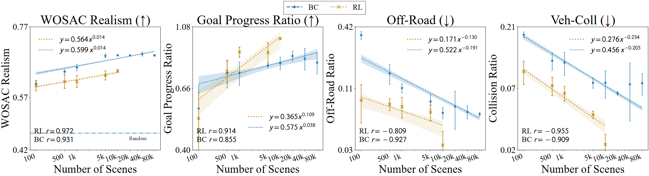
Driving logs are heavily biased toward nominal straight-driving scenes, and a model can score well while largely neglecting information beyond the ego state.12 BC and RL do improve under closed-loop evaluation, but those gains do not by themselves show that the policies have internalized prediction and planning.
Swipe to read the panels · Enlarge for the full figure
These scores leave open whether the closed-loop gains reflect stronger prediction and planning or heuristics that succeed in nominal scenes.
A robust driving policy should respond sensibly to changes in its surroundings, distinguish relevant from irrelevant vehicles, and maintain plans for safety-critical interactions.
A slowing or newly introduced lead vehicle should induce deceleration, while removing a lead vehicle should allow the ego to accelerate.
The policy should attend to nearby vehicles that may affect its future path, rather than to distant vehicles with little relevance to the ego plan.
The policy should remain prepared for unexpected interactions, such as an abrupt cut-in, rather than only for the nominal scenes that dominate the data.
We use linear probing, perturbed closed-loop simulation, and causal interventions to examine how prediction and planning are accessible in behavior cloning and reinforcement learning policies.
Linear probes measure information that is linearly accessible from the policy’s representation. We investigate three connected questions.
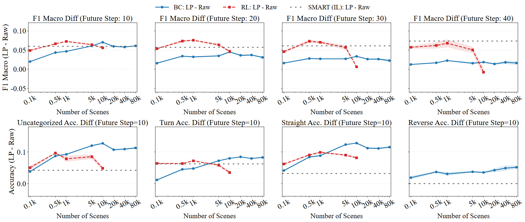
For BC, probing gains increase up to about 10K scenes and then largely plateau. RL does not improve monotonically: from 5K to 10K scenes, driving and ego-plan probing improve while surrounding-vehicle probing weakens.
Swipe to read the panels · Enlarge for the full figure
The gains are uneven across trajectory types. BC improves more for Straight and Uncategorized futures than for Turn and Reverse cases. Relative probing gain, LP − Raw, measures the additional linearly accessible information beyond a probe trained directly on raw input.
Swipe to read the panels · Enlarge for the full figure
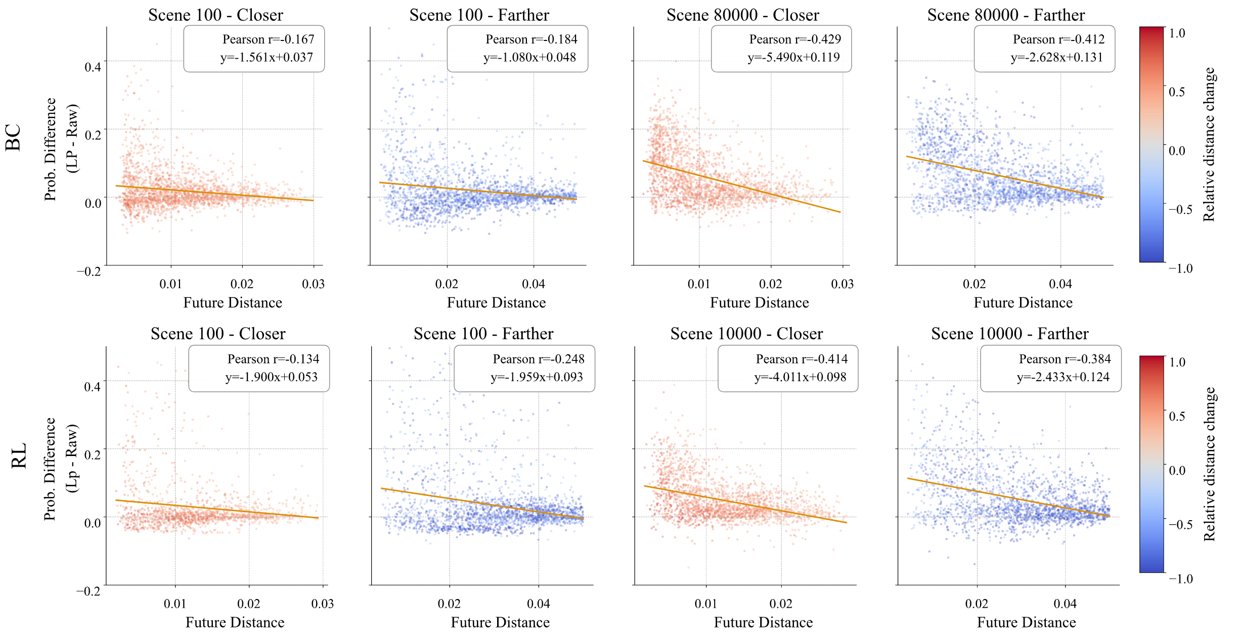
At 100 scenes, the linear probe advantage is only weakly associated with future ego–other distance. At 10K and 80K scenes, the association becomes more negative: the probing advantage is stronger for vehicles that remain close. Among nearby vehicles, however, approaching and receding vehicles have similar probing signals. Scaling increasingly separates distant from nearby vehicles, but it does not clearly distinguish which nearby vehicle will become most interaction-relevant.
If a policy uses surrounding-vehicle information selectively, removing distant vehicles should have less effect than removing nearby vehicles. We progressively remove surrounding vehicles in nearest-first and farthest-first order.
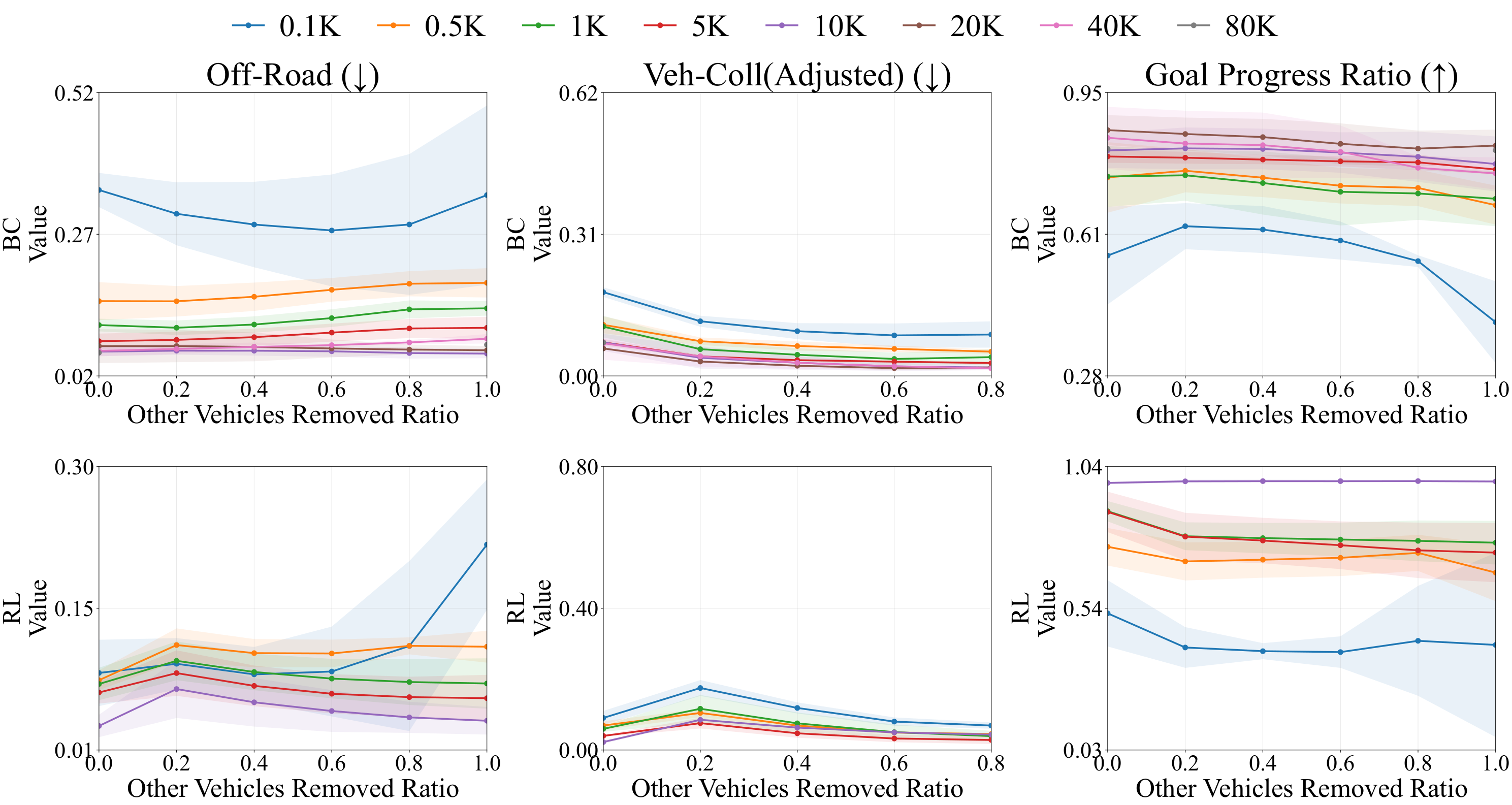
Swipe to read the panels · Enlarge for the full figure
Removing nearby vehicles increasingly degrades goal progress at high removal ratios, even as adjusted vehicle-collision rate decreases.
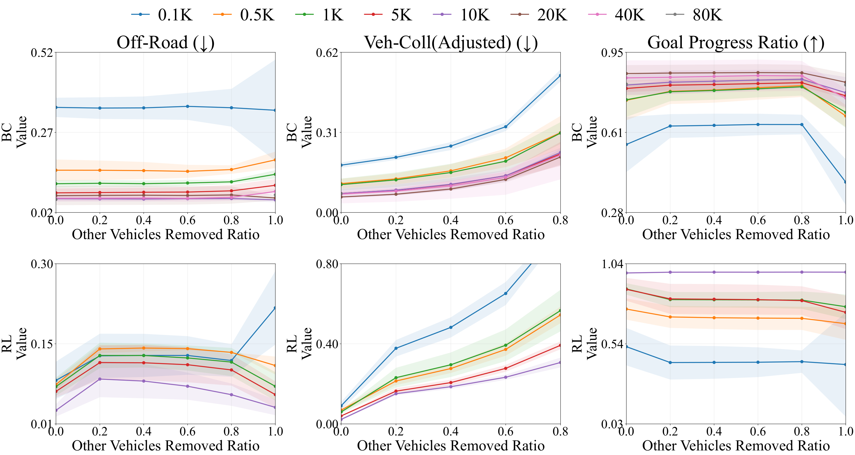
Swipe to read the panels · Enlarge for the full figure
Removing distant vehicles has little effect on goal progress through high removal ratios, indicating relative insensitivity to distant-agent context.
Adjusted vehicle-collision rate = Veh-Coll / (1 − p), where p is the fraction of surrounding vehicles removed. This rate is normalized by the remaining-vehicle ratio and is undefined at p = 1.
Nearest-first removal suggests brittleness to the removal of nearby-agent context rather than increased interaction difficulty. Naturally occurring single-AV scenes already perform worse than normal scenes, and removing vehicles from an originally interactive scene causes a further decline.
Together, these results suggest limited generalization to reduced-interaction settings and sensitivity to nearby-agent context, rather than a general spurious reliance on surrounding vehicles.
Early anticipation of a dangerous interaction would appear as a strong positive probing signal at 40, 30, or 20 steps before collision. For both BC and RL, the strongest signal appears mainly in the final 10 steps and is concentrated near the ego.
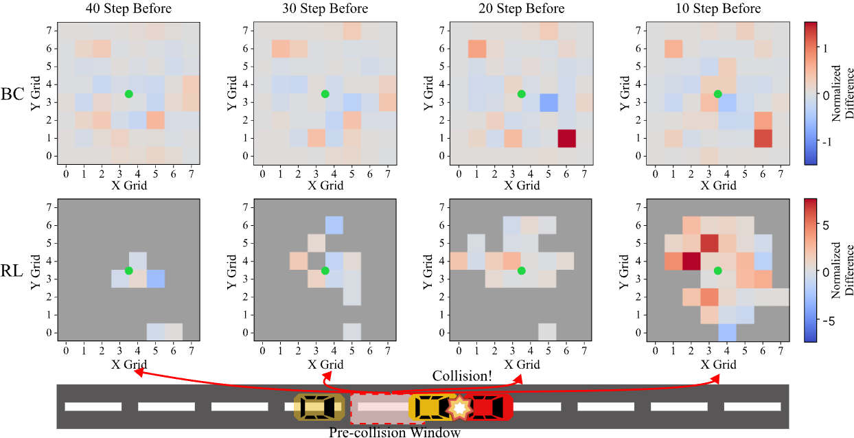
Swipe to read the panels · Enlarge for the full figure
RL collisions are much rarer, leaving fewer samples and more filtered regions, but the same late peak remains. In these episodes, the relevant vehicle becomes strongly linearly decodable only shortly before collision.
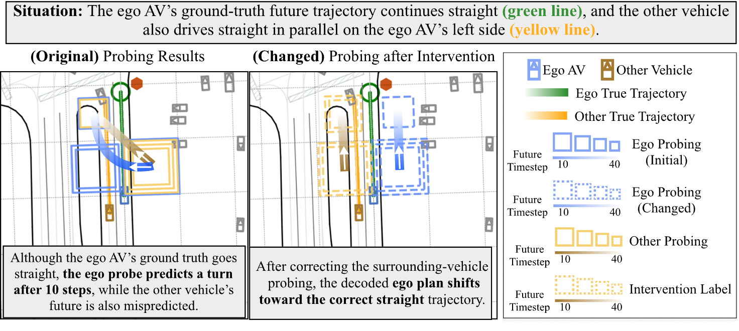
We intervene on the surrounding-vehicle representation along a linear probe direction and propagate the modified representation through the policy. Adaptiveness and recovery test how that intervention affects ego behavior. Both settings are compared with magnitude-matched random controls.
We induce surrounding-vehicle predictions that conflict with the ego’s decoded path. Positive CAP indicates increased separation from that induced trajectory.
We correct an erroneous surrounding-vehicle prediction toward its logged future. Positive GPG indicates that goal progress improves relative to the unmodified policy.
| Metric | Semantic intervention | Random control |
|---|---|---|
| BC Behavior cloning | ||
| Separation from the induced conflict CAP · adaptiveness | 2.61 m | 0.92 m |
| Ego-trajectory change ADE · adaptiveness | 3.67 m | 1.91 m |
| Low-progress recovery Baseline goal progress ≤ 0.5; changed outcomes only | +21.8 ppn = 431 | +9.9 ppn = 430 |
| RL Reinforcement learning | ||
| Separation from the induced conflict CAP · adaptiveness | 0.022 m | 0.010 m |
| Ego-trajectory change ADE · adaptiveness | 0.280 m | 0.357 m |
| Low-progress recovery Baseline goal progress ≤ 0.5; changed outcomes only | +41.3 ppn = 29 | +31.3 ppn = 39 |
pp = percentage points. CAP and ADE are reported in meters; recovery is the change in goal-progress ratio. Random controls are magnitude-matched. §3.5 · Tables 13–15
Low-progress recovery rows follow Appendix G, Table 14(c,d): baseline goal progress is at most 0.5, and only scenes whose outcomes change are included. The BC and RL subsets are not the same as their full recovery evaluation sets. BC and RL GPG is measured in closed-loop simulation; the accompanying example figures show linear probe readouts.
For BC, the semantic intervention moves the ego trajectory away from the induced conflict and improves goal progress, including in low-progress scenes. For RL, the intervention alters the prediction-related representation in the intended direction, but that change does not consistently propagate to ego planning.
Improved recovery does not imply uniform safety gains. For BC, collision and off-road rates increase slightly despite better goal progress.
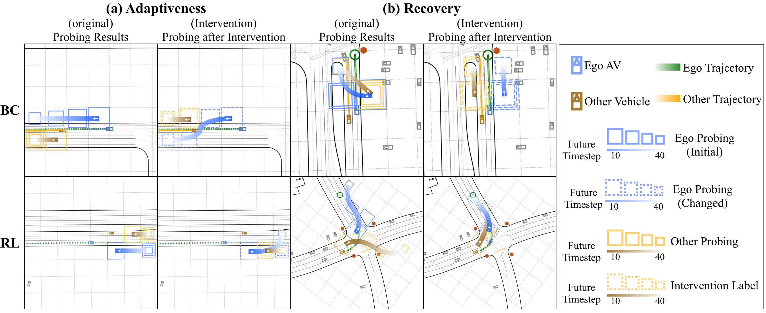
Swipe to read the panels · Enlarge for the full figure
@article{jeon2026probing,
  title={What Probing Reveals about Autonomous Driving:
         Linking Internal Prediction Errors to Ego Planning},
  author={Jeon, Hyeonchang and Kim, Kyungbeom and
          Vinitsky, Eugene and Kim, Kyung-Joong},
  journal={arXiv preprint arXiv:2606.31106},
  year={2026}
}